Plotting

This page demonstrates all plots which are available through this package. Note that the API reference for each method is available here.

Demo Data

First, we’ll load some example data:

[1]:

from pathlib import Path
import sys
sys.path.append('../')  # not necessary when the library is installed
from ParticlePhaseSpace import DataLoaders
from ParticlePhaseSpace import PhaseSpace

test_data_loc = Path(r'../tests/test_data/coll_PhaseSpace_xAng_0.00_yAng_0.00_angular_error_0.0.phsp').absolute()
ps_data = DataLoaders.Load_TopasData(test_data_loc)
PS = PhaseSpace(ps_data)

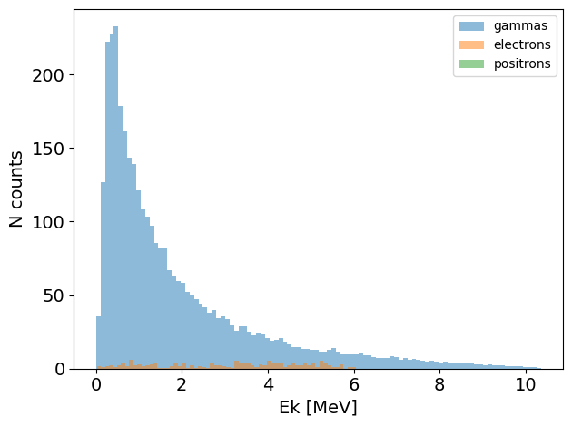
energy_hist_1D

[2]:

PS.plot.energy_hist_1D()

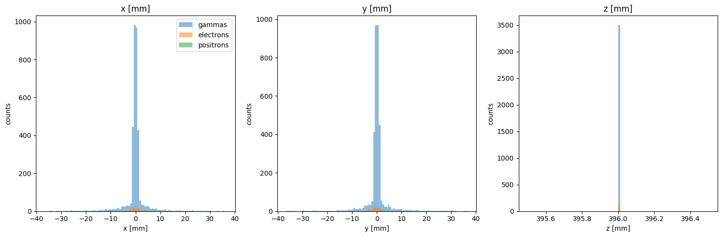
position_hist_1D

[3]:

PS.plot.position_hist_1D()

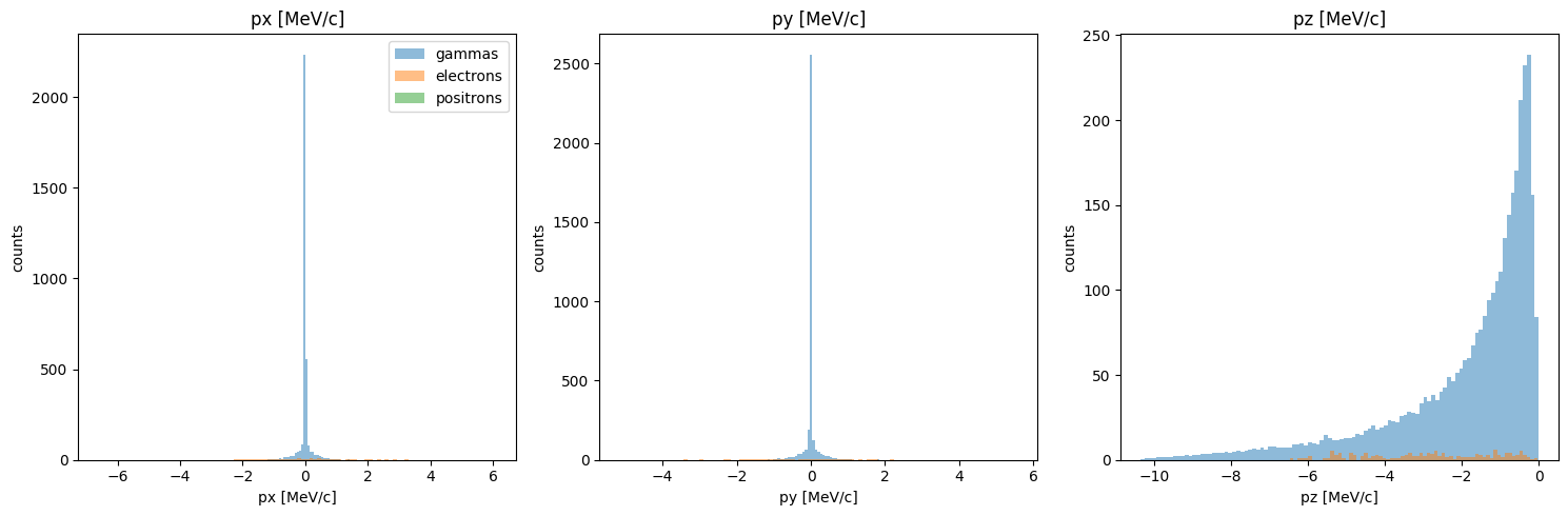
momentum_hist_1D

[4]:

PS.plot.momentum_hist_1D()

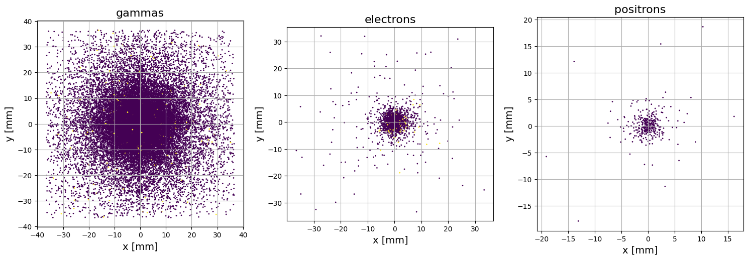
particle_positions_scatter_2D

[5]:

PS.plot.particle_positions_scatter_2D()

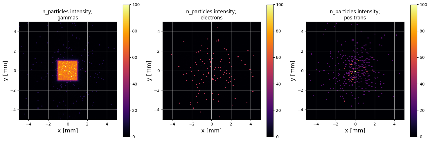
particle_positions_hist_2D

[6]:

PS.plot.particle_positions_hist_2D(xlim=[-5, 5], ylim=[-5, 5])

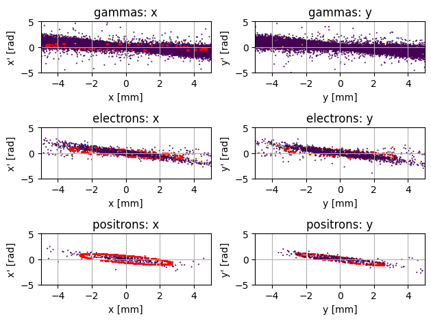
transverse_trace_space_scatter_2D

[7]:

PS.plot.transverse_trace_space_scatter_2D(xlim=[-5, 5], ylim=[-5, 5])

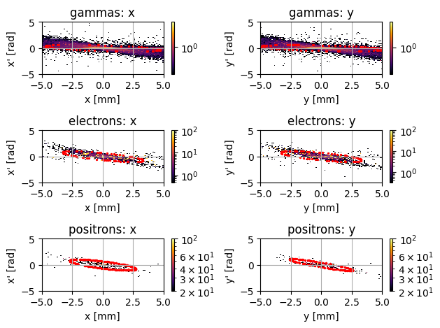
transverse_trace_space_hist_2D

[8]:

PS.plot.transverse_trace_space_hist_2D(xlim=[-5, 5], ylim=[-5, 5])

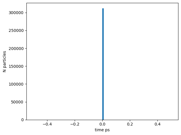
n_particles_v_time

(note: this demo data only has one time point so this doesn’t look particularly impressive!)

[9]:

PS.plot.n_particles_v_time()

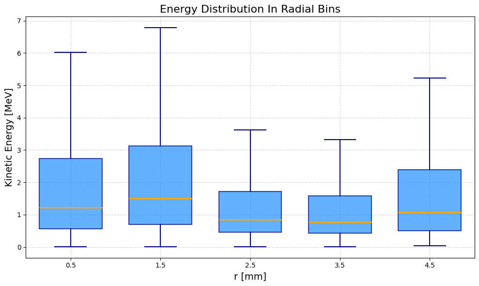
radial_energy_boxplot

[10]:

PS.plot.radial_energy_boxplot(rlim=[0, 5])

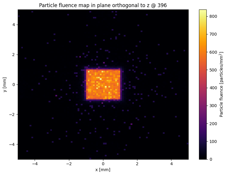
fluence_map_2D

To plot the particle fluence:

[11]:

PS.plot.fluence_map_2D(quantity="particle", at=396, xlim=[-5, 5], ylim=[-5, 5])

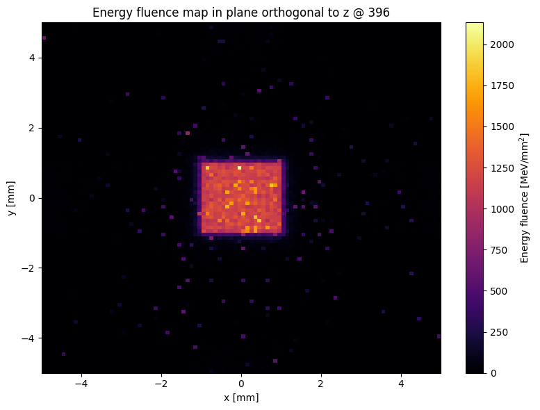
To plot the energy fluence:

[12]:

PS.plot.fluence_map_2D(quantity="energy", at=396, xlim=[-5, 5], ylim=[-5, 5])

[ ]: